Run each scheme
We test the following:
running the model with default case (all schemes)
plot methods for
Modelclassxarray.Datasetoutputplots for output
xarray.Datasets
import matplotlib as mpl
import matplotlib.pyplot as plt
import numpy as np
import pandas as pd
import xarray as xr

import crt1d as crt
Examine available schemes
crt.print_config()
scheme IDs available: 2s, 4s, bf, bl, g77, n79, zq, zq_pa
crt1d base dir
    /home/docs/checkouts/readthedocs.org/user_builds/crt1d/envs/latest/lib/python3.11/site-packages/crt1d
looking for input data for provided cases in
    /home/docs/checkouts/readthedocs.org/user_builds/crt1d/envs/latest/lib/python3.11/site-packages/crt1d/data
df_schemes = pd.DataFrame(crt.solvers.AVAILABLE_SCHEMES).T

BL_args = set(a for a in df_schemes.loc[df_schemes.name == "bl"].args.values[0])
df_schemes["args_minus_BL"] = df_schemes["args"].apply(
    lambda x: list(set(x).symmetric_difference(BL_args))
)

print("B-L args:", ", ".join(BL_args))

df_schemes.drop(columns=["args", "solver"])  # solver memory address not very informative
B-L args: I_dr0_all, lai, psi, I_df0_all, leaf_t, leaf_r, K_b_fn
| module_name | name | short_name | long_name | options | args_minus_BL | |
|---|---|---|---|---|---|---|
| 2s | _solve_2s | 2s | 2s | Dickinson–Sellers two-stream | [] | [mla, soil_r, G_fn] |
| 4s | _solve_4s | 4s | 4s | Tian et al. four-stream | [mu_s] | [soil_r, G_fn] |
| bf | _solve_bf | bf | BF | Bodin & Franklin improved Goudriaan | [] | [soil_r] |
| bl | _solve_bl | bl | B–L | Beer–Lambert | [] | [] |
| g77 | _solve_g77 | g77 | G77 | Goudriaan (1977) | [] | [soil_r] |
| n79 | _solve_n79 | n79 | N79 | Norman (1979) | [tau_d_method] | [soil_r] |
| zq | _solve_zq | zq | ZQ | Zhao & Qualls multi-scattering | [] | [soil_r, G_fn] |
| zq_pa | _solve_zq_pa | zq_pa | ZQ-pA | Zhao & Qualls multi-scattering (pyAPES) | [] | [clump, soil_r] |
👆 We see that all schemes take at least one more argument than what B–L (bl) requires. The B–L scheme makes the black soil assumption and so does not need soil_r. Additionally, some schemes have some parameters on top of the required arguments (column options).
Run
Run the default case (which is loaded automatically when model object is created).
scheme_names = list(crt.solvers.AVAILABLE_SCHEMES)

ms = []
for scheme_name in scheme_names:  # run all available
    m = crt.Model(scheme_name, nlayers=60).run().calc_absorption()
    ms.append(m)

dsets = [m.to_xr() for m in ms]
Examine default case
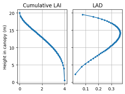
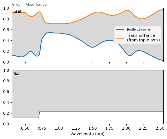
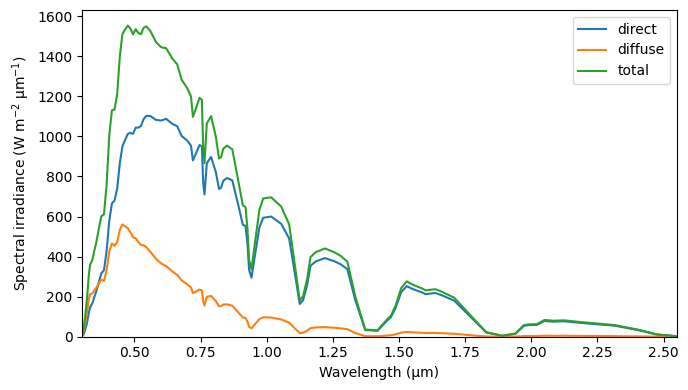
We plot the leaf area profile, leaf/soil optical property spectra, and top-of-canopy spectral, using the plotting methods attached to the Model instance.
m0 = ms[0]

m0.plot_canopy()
m0.plot_leafsoil_spectra()
m0.plot_toc_spectra()
Compare results
In crt1d.diagnostics, there are some functions that can be used to compare a set of model output datasets.
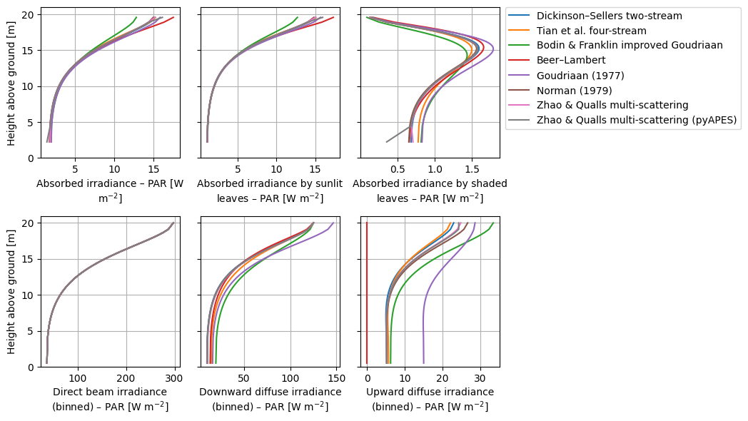
Plots – single band
We demonstrate the function crt1d.diagnostics.plot_compare_band().
crt.diagnostics.plot_compare_band(dsets, band_name="PAR", marker=None)
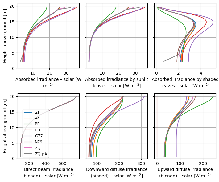
crt.diagnostics.plot_compare_band(
    dsets, band_name="solar", marker=None,
    legend_outside=False, ds_labels="scheme_short_name"
)
Optionally, we can compare to a reference, in order to better see the differences among schemes.
crt.diagnostics.plot_compare_band(
    dsets, band_name="solar", marker=None,
    legend_outside=False, ds_labels="scheme_short_name",
    ref="2s"
)
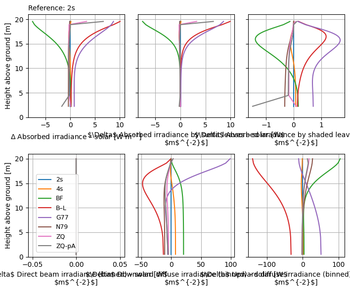
With ref_relative=True, the differences are computed as relative error (indicated by \(\Delta_r\)). Otherwise (above), they are absolute (indicated by \(\Delta\)). Relative error allows us to better see the differences in the lower regions of the canopy where there is less light.
crt.diagnostics.plot_compare_band(
    dsets[1:], band_name="solar", marker=None,
    legend_outside=False, ds_labels="scheme_short_name",
    ref=dsets[0], ref_relative=True, ref_label="a fancy 2s run"
)
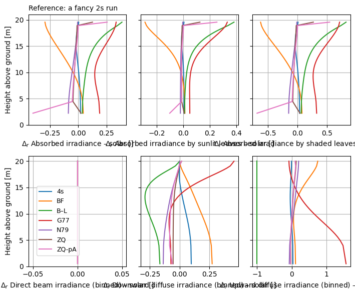
👆 Note that the reference does not have to belong to dsets if passed as an xarray.Dataset.
Plots – spectra
We demonstrate the function crt1d.diagnostics.plot_compare_spectra().
crt.diagnostics.plot_compare_spectra(dsets)
👆 It is hard to see differences this way. Like with crt1d.diagnostics.plot_compare_band(), we have some options to help illuminate the differences.
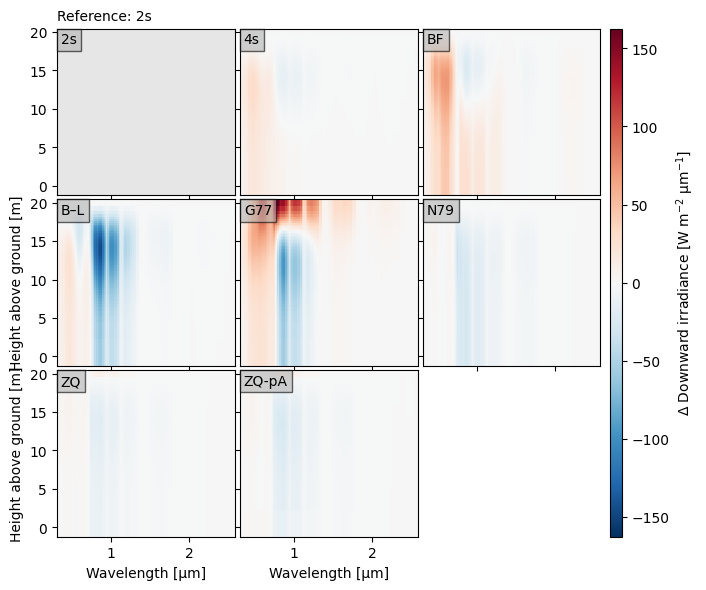
crt.diagnostics.plot_compare_spectra(dsets, ref="2s")
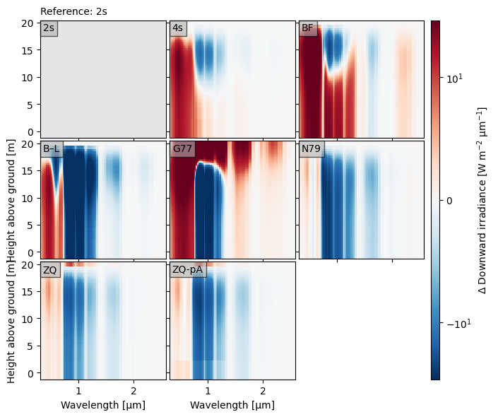
crt.diagnostics.plot_compare_spectra(
dsets,
ref="2s",
norm=mpl.colors.SymLogNorm(10, base=10),
)
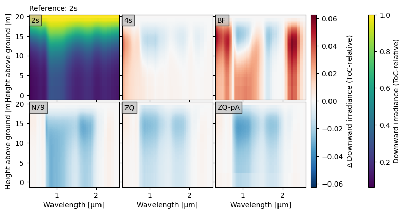
Optionally, we can plot the reference spectra like normal, so that it is clear what the differences are relative to. In the plot below, we highlight how the spectrum changes from top-of-canopy to below by using the toc_relative option.
crt.diagnostics.plot_compare_spectra(
    dsets[:3] + dsets[5:],
    toc_relative=True,
    ref="2s", ref_plot=True
)
Plots – xarray
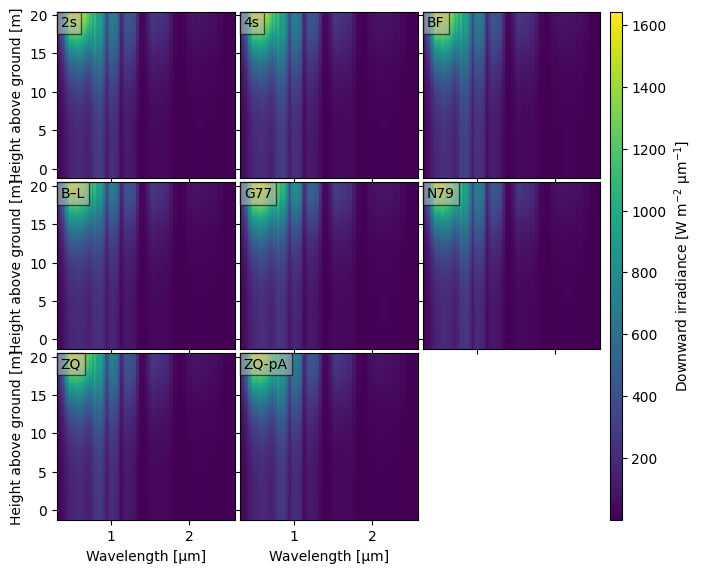
Note that with the magic of xarray.plot.FacetGrid (examples here), we can make similar plots to the above.
xr.concat(
    [ds["I_d"] for ds in dsets],
    dim=xr.DataArray(name="exp", dims="exp", data=scheme_names)
).plot(
    x="wl", y="z", col="exp", col_wrap=3
);
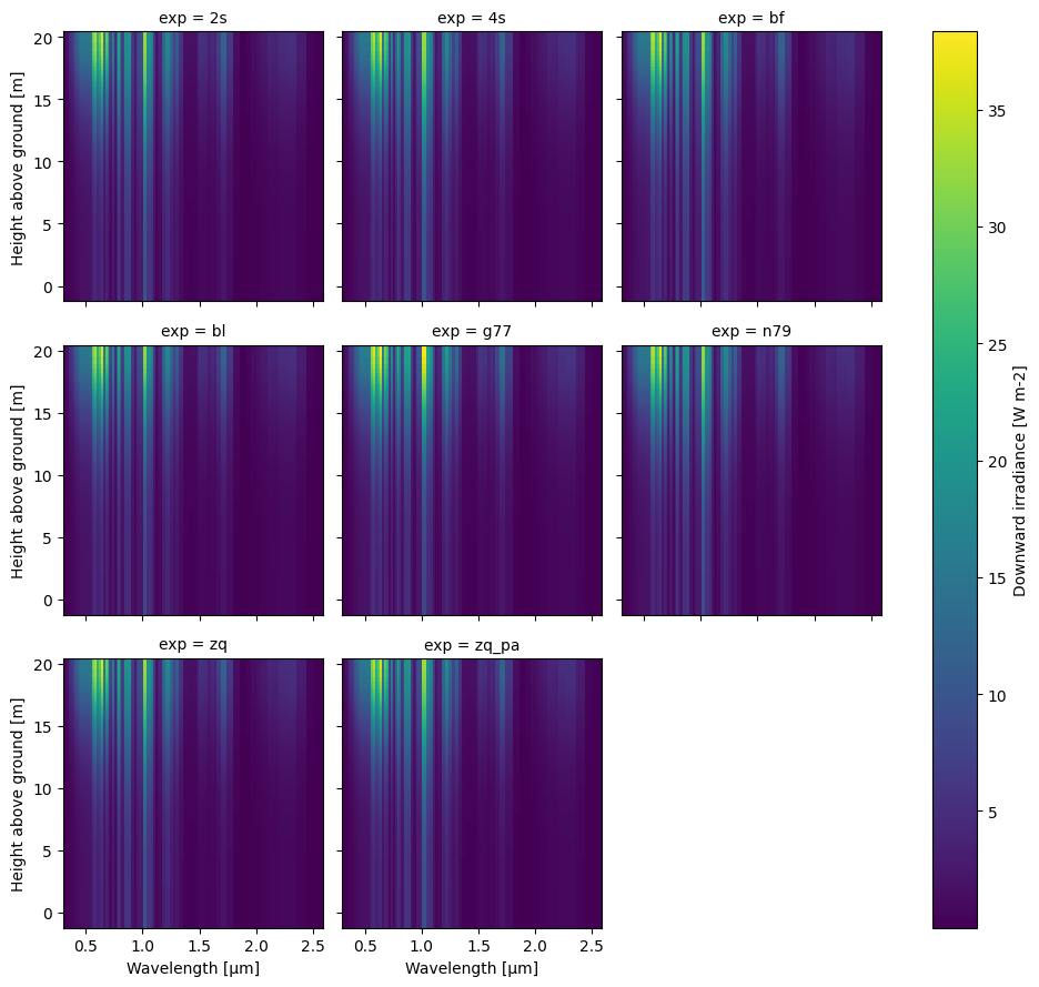
👆 Merging the whole dataset is a bit more awkward since we have dataset attribute conflicts (though we can use combine_attrs='drop_conflicts' if we have xarray v0.17+) and some datasets have extra variables. Above we get around these problems by merging a selected variable instead.
Other diagnostic tools
crt.diagnostics.compare_ebal(dsets).astype(float).round(3)
| incoming | outgoing (reflected) | soil absorbed | layerwise abs sum | in-out-soil | canopy abs | |
|---|---|---|---|---|---|---|
| 2s | 982.509 | 140.117 | 139.381 | 703.011 | 703.011 | 703.011 |
| 4s | 982.509 | 138.916 | 145.774 | 697.820 | 697.820 | 697.820 |
| bf | 982.509 | 244.540 | 156.812 | 581.157 | 581.157 | 581.157 |
| bl | 982.509 | 0.000 | 159.327 | 823.182 | 823.182 | 823.182 |
| g77 | 1081.284 | 128.517 | 82.768 | 869.999 | 869.999 | 869.999 |
| n79 | 982.509 | 167.410 | 131.162 | 683.937 | 683.937 | 683.937 |
| zq | 986.077 | 157.436 | 136.143 | 692.498 | 692.498 | 692.498 |
| zq_pa | 985.920 | 153.011 | 135.760 | 697.149 | 697.149 | 697.149 |
Model output datasets
See the variables page for more information about the output variables.
dsets[0]
<xarray.Dataset> Size: 616kB
Dimensions:   (z: 60, wl: 107, zm: 59, wle: 108)
Coordinates:
  * z         (z) float64 480B 0.5 3.966 4.922 5.609 ... 18.34 18.68 19.11 20.0
  * wl        (wl) float64 856B 0.3025 0.3075 0.3125 0.3175 ... 2.405 2.475 2.55
  * zm        (zm) float64 472B 2.233 4.444 5.266 5.888 ... 18.51 18.89 19.55
  * wle       (wle) float64 864B 0.3 0.305 0.31 0.315 0.32 ... 2.36 2.45 2.5 2.6
Data variables: (12/21)
    I_dr      (z, wl) float64 51kB 0.001447 0.006402 0.01758 ... 0.544 0.2569
    I_df_d    (z, wl) float64 51kB 0.001012 0.004119 ... 0.02288 0.009896
    I_df_u    (z, wl) float64 51kB 0.0002705 0.001157 ... 0.01064 0.001819
    F         (z, wl) float64 51kB 0.004104 0.01737 0.04577 ... 0.646 0.2969
    I_d       (z, wl) float64 51kB 0.002459 0.01052 0.02803 ... 0.5669 0.2668
    dwl       (wl) float64 856B 0.005 0.005 0.005 0.005 ... 0.09 0.09 0.05 0.1
    ...        ...
    laim      (zm) float64 472B 3.966 3.898 3.831 3.763 ... 0.1695 0.1017 0.0339
    f_slm     (zm) float64 472B 0.1267 0.1313 0.136 ... 0.9155 0.9484 0.9825
    psi       float64 8B 0.3491
    sza       float64 8B 20.0
    G         float64 8B 0.4894
    K_b       float64 8B 0.5208
Attributes:
    info:
    scheme_name:        2s
    scheme_long_name:   Dickinson–Sellers two-stream
    scheme_short_name:  2s
crt1d_version: 0.1.dev90+g61e599119dsets[0]["zm"]
<xarray.DataArray 'zm' (zm: 59)> Size: 472B
array([ 2.233243,  4.444249,  5.265545,  5.888072,  6.406822,  6.859524,
        7.265752,  7.637189,  7.981456,  8.303839,  8.608181,  8.897375,
        9.173663,  9.438827,  9.694307,  9.94129 , 10.180769, 10.413585,
       10.640457, 10.862012, 11.078795, 11.29129 , 11.499927, 11.705094,
       11.907143, 12.106395, 12.303146, 12.497673, 12.690234, 12.881074,
       13.070427, 13.258519, 13.445569, 13.631793, 13.817406, 14.002623,
       14.187664, 14.372752, 14.558122, 14.744021, 14.93071 , 15.118471,
       15.307616, 15.498485, 15.691464, 15.886992, 16.085578, 16.287821,
       16.494442, 16.706323, 16.924573, 17.150628, 17.386407, 17.6346  ,
       17.899194, 18.186622, 18.508678, 18.892952, 19.552798])
Coordinates:
* zm (zm) float64 472B 2.233 4.444 5.266 5.888 ... 18.51 18.89 19.55
Attributes:
long_name: Height above ground
units: m# Some schemes generate extra outputs (in addition to the required)
ms[scheme_names.index("zq")].out_extra
{'I_df_d_ss_scheme': array([[0.0011174 , 0.00453624, 0.01147541, ..., 0.05775764, 0.0050126 ,
         0.00090819],
        [0.0011775 , 0.00477837, 0.01208304, ..., 0.0591903 , 0.00514565,
         0.00093767],
        [0.00124104, 0.00503426, 0.01272508, ..., 0.06067554, 0.00528461,
         0.00096874],
        ...,
        [0.02539346, 0.10176728, 0.25397733, ..., 0.15556606, 0.02216082,
         0.00902544],
        [0.02686378, 0.10764841, 0.26862401, ..., 0.15305175, 0.02250769,
         0.00944879],
        [0.02843666, 0.11394001, 0.28429375, ..., 0.15073189, 0.02287754,
         0.00989642]], shape=(60, 107)),
 'I_df_u_ss_scheme': array([[0.00015918, 0.0007042 , 0.0019335 , ..., 0.08350631, 0.0152426 ,
         0.00719909],
        [0.0002663 , 0.00113788, 0.00302736, ..., 0.09210497, 0.0155031 ,
         0.00696519],
        [0.00026468, 0.00112976, 0.00300279, ..., 0.08850114, 0.01472284,
         0.00655977],
        ...,
        [0.00186484, 0.00761463, 0.01937933, ..., 0.11479556, 0.0107946 ,
         0.00193982],
        [0.00196119, 0.00800401, 0.02035995, ..., 0.11827098, 0.01112857,
         0.00199167],
        [0.0020628 , 0.00841452, 0.02139341, ..., 0.12186427, 0.01147647,
         0.00204659]], shape=(60, 107)),
 'F_ss_scheme': array([[0.00409313, 0.0172935 , 0.04552318, ..., 0.67748594, 0.11260302,
         0.05026394],
        [0.00448293, 0.01888997, 0.04959841, ..., 0.71174317, 0.11598109,
         0.05107883],
        [0.00466408, 0.01963916, 0.05152978, ..., 0.7222107 , 0.11738256,
         0.05159781],
        ...,
        [0.06603977, 0.26974079, 0.68668028, ..., 3.49608316, 0.60535961,
         0.27671251],
        [0.06958724, 0.28411388, 0.72296522, ..., 3.60421941, 0.6261088 ,
         0.28681965],
        [0.07336524, 0.29941604, 0.76158274, ..., 3.71679759, 0.64762855,
         0.29731055]], shape=(60, 107))}