External spectra sources
crt1d comes with some functions that facilitate easy generation of leaf optical property and top-of-canopy irradiance spectra using external programs. These can be found in module crt1d.data.
import matplotlib as mpl
import matplotlib.pyplot as plt
import numpy as np
import pandas as pd
import xarray as xr

import crt1d as crt
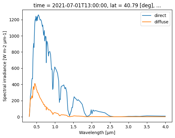
SPCTRAL2
crt1d.data.solar_sp2() runs SPCTRAL2 (via SolarUtils) and saves the results to an xarray.Dataset.
Example
Walker Building in the summer around local solar noon.
lat = 40.793275995962944
lon = -77.86686570952304
dt0 = pd.Timestamp("2021/07/01 13:00")
utcoffset = -4  # EDT

ds = crt.data.solar_sp2(dt0, lat, lon, utcoffset=utcoffset)
ds
<xarray.Dataset> Size: 2kB
Dimensions:  (wl: 122)
Coordinates:
  * wl       (wl) float32 488B 0.3 0.305 0.31 0.315 0.32 ... 3.6 3.7 3.8 3.9 4.0
    time     datetime64[us] 8B 2021-07-01T13:00:00
    lat      float64 8B 40.79
    lon      float64 8B -77.87
Data variables:
    SI_dr    (wl) float64 976B 2.323 18.16 47.95 95.28 ... 8.518 7.66 7.589
    SI_df    (wl) float32 488B 3.502 24.66 59.09 ... 0.09369 0.08087 0.07696
    SI_et    (wl) float32 488B 518.0 539.7 601.3 669.6 ... 10.05 9.183 8.313
    sza      float64 8B 18.03
    saa      float64 8B 168.5
inc float64 8B 18.03fig, ax = plt.subplots()
ds.SI_dr.plot(ax=ax, label="direct")
ds.SI_df.plot(ax=ax, label="diffuse")
ax.set(ylabel=f"Spectral irradiance [{ds.SI_dr.units}]")
ax.legend();
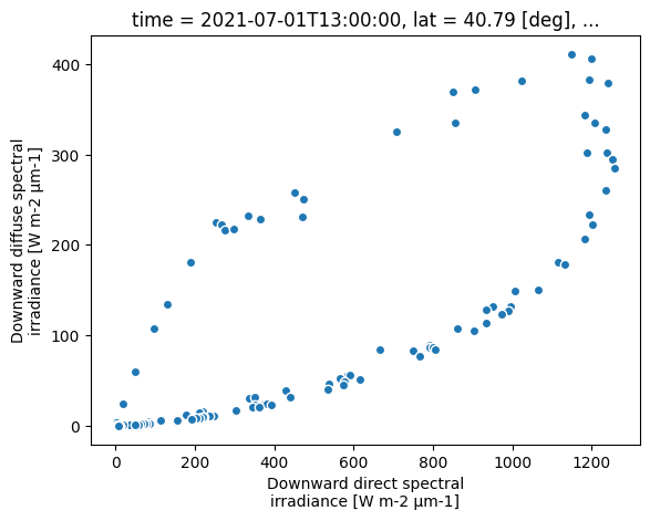
ds.plot.scatter(x="SI_dr", y="SI_df");
Variations
Time of day
dts = pd.date_range("2021/07/01 10:00", "2021/07/01 20:00", freq="15min")

ds = xr.concat(
    [crt.data.solar_sp2(dt, lat, lon, utcoffset=utcoffset) for dt in dts],
    dim="time"
)

def plot(ds, x=None):
    if x is None:
        x = list(ds.dims)[0]

    fig, axs = plt.subplots(2, 2, figsize=(9, 6))
    ax1, ax2, ax3, ax4 = axs.flat

    ds.SI_dr.plot(x=x, ax=ax1)
    ds.SI_df.plot(x=x, ax=ax2)

    norm = mpl.colors.LogNorm(vmin=1e-10)
    (ds.SI_dr / ds.SI_dr.isel({x: 0})).plot(x=x, ax=ax3, norm=norm)
    (ds.SI_df / ds.SI_df.isel({x: 0})).plot(x=x, ax=ax4, norm=norm)

    fig.tight_layout()

plot(ds)
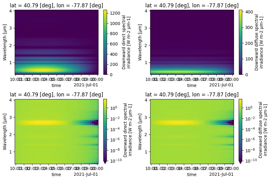
👆 The second row shows how the spectrum shape changes since the first time shown. It seems that, for the most part, the spectrum shape doesn’t change much with time of day on a given day in this model (except around 2.7 μm).
Parameters
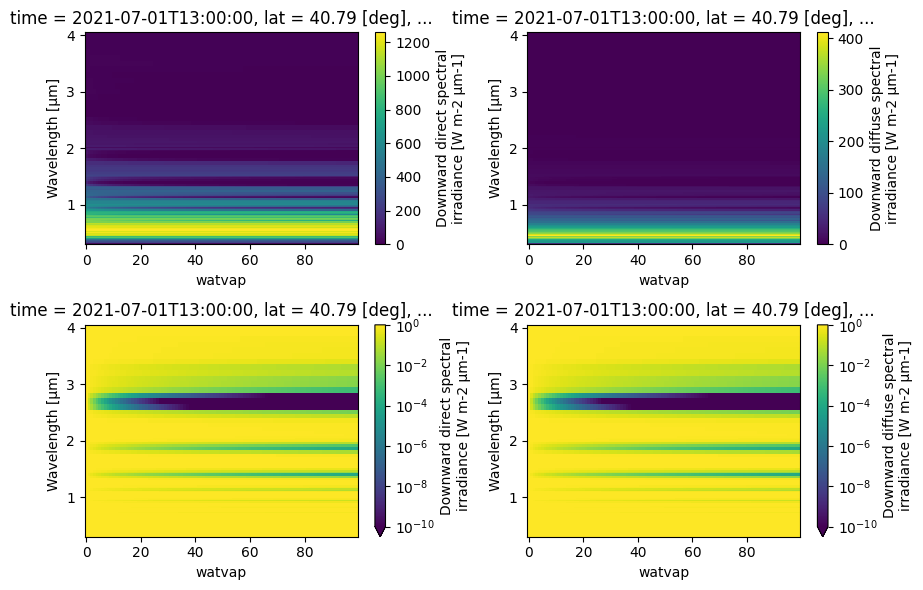
watvaps = np.linspace(0.1, 10., 100)

ds = xr.concat(
    [crt.data.solar_sp2(dt0, lat, lon, utcoffset=utcoffset, watvap=watvap) for watvap in watvaps],
    dim="watvap"
)

plot(ds)
# TODO: others
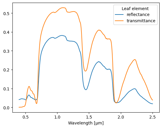
PROSPECT-5
crt1d.data.leaf_ps5() runs PROSPECT-5 (via Python PROSAIL) and saves the results to an xarray.Dataset.
ds = crt.data.leaf_ps5()
ds
<xarray.Dataset> Size: 50kB
Dimensions:  (wl: 2101)
Coordinates:
  * wl       (wl) float64 17kB 0.4 0.401 0.402 0.403 ... 2.497 2.498 2.499 2.5
Data variables:
    rl       (wl) float64 17kB 0.04099 0.04103 0.04106 ... 0.01878 0.0188
    tl       (wl) float64 17kB 0.0003881 0.0003982 0.0004079 ... 0.03852 0.0385
    n        float64 8B 1.2
    cab      float64 8B 30.0
    car      float64 8B 10.0
    cbr      float64 8B 1.0
    ewt      float64 8B 0.015
lma float64 8B 0.009fig, ax = plt.subplots()
ds.rl.plot(ax=ax, label="reflectance")
ds.tl.plot(ax=ax, label="transmittance")
ax.set(ylabel="")
ax.legend(title="Leaf element");