Binning spectra
Module crt1d.spectra provides some tools for working with spectra.
By binning or smearing spectra, we can use spectra together that were originally on different grids.
Also, we can decrease canopy RT computational time by reducing spectral resolution.
import matplotlib.pyplot as plt
import numpy as np
from scipy import stats

import crt1d as crt
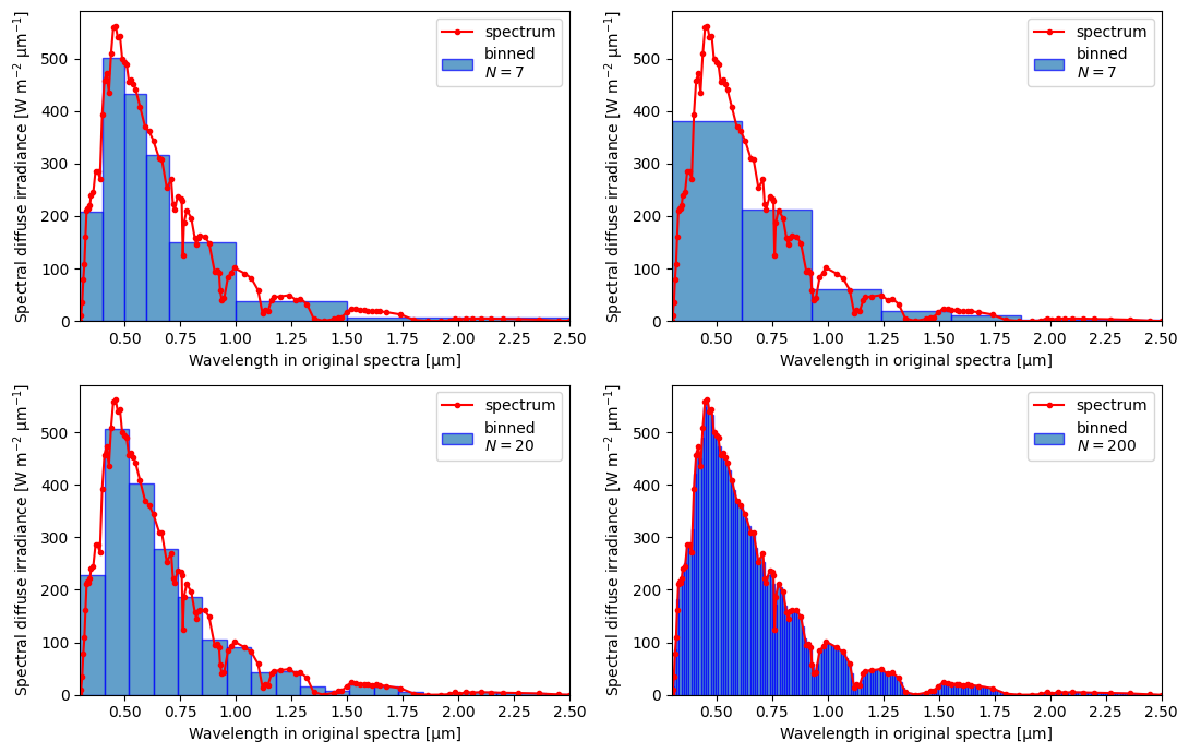
Solar
Although the main purpose of the “smear” functions is to provide the ability to go to lower spectral resolution while conserving certain properties, they also work as interpolators when a higher resolution grid is used.
Note
The bins do not have to be equal-width—variable grid will also work!
ds0 = crt.data.load_default_sp2()
ds0
<xarray.Dataset> Size: 8kB
Dimensions:  (wl0: 122, wl: 121, wle: 122)
Coordinates:
  * wl0      (wl0) float64 976B 0.3 0.305 0.31 0.315 0.32 ... 3.7 3.8 3.9 4.0
  * wl       (wl) float64 968B 0.3025 0.3075 0.3125 0.3175 ... 3.75 3.85 3.95
  * wle      (wle) float64 976B 0.3 0.305 0.31 0.315 0.32 ... 3.7 3.8 3.9 4.0
Data variables:
    SI_dr    (wl0) float64 976B 0.26 4.388 16.17 40.28 ... 9.046 8.127 8.219
    SI_df    (wl0) float64 976B 0.7224 10.65 34.92 ... 0.2995 0.2616 0.2653
    I_dr     (wl) float64 968B 0.01162 0.05141 0.1411 ... 0.9325 0.8587 0.8173
    I_df     (wl) float64 968B 0.02844 0.1139 0.2843 ... 0.03113 0.02806 0.02635
dwl (wl) float64 968B 0.005 0.005 0.005 0.005 0.005 ... 0.1 0.1 0.1 0.1binss = [
[0.3, 0.4, 0.5, 0.6, 0.7, 1.0, 1.5, 2.5], # variable dx is supported
np.linspace(0.3, 2.5, 8),
np.linspace(0.3, 2.5, 21),
np.linspace(0.3, 2.5, 201),
]
fig, ax = plt.subplots(2, 2, figsize=(11, 7))
for bins, ax in zip(binss, ax.flat):
# The spectral variables have coord `wl0`
crt.spectra.plot_binned_ds(ds0, crt.spectra.smear(ds0, bins, x="wl0"), yname="SI_df", xtight="bins", ax=ax)
Warning
Irradiance (W m-2) should not be smeared directly (as we see below). Instead we use a special routine to calculate in-bin irradiance by smearing spectral irradiance (W m-2 μm-1).
If we smear irradiance directly, the total irradiance is essentially proportional to the number of bins used. For equal-width bins, it turns out to be exactly proportional.
tot0 = ds0.I_dr.sum().values
tot = []
nbands = np.arange(1, 200, 10)
for n in nbands:
    tot.append(crt.spectra.smear(ds0, np.linspace(0.3, 4.0, n)).I_dr.sum().values)

res = stats.linregress(nbands, tot)

fig, ax = plt.subplots()
ax.plot(nbands, tot, ".-")
ax.text(0.03, 0.96, f"Original total: {tot0:.4g}\nr$^2 = {res.rvalue**2:.3f}$", ha="left", va="top", transform=ax.transAxes)
ax.set(xlabel="# of bands", ylabel="Total irradiance [W m-2]");
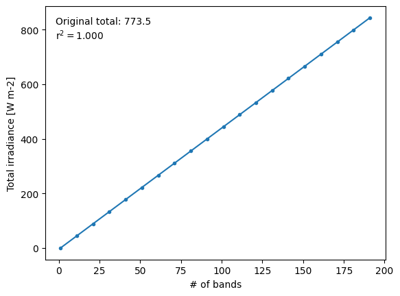
Instead, for computing irradiance in bins, crt1d.spectra.smear_si() can be used for convenience. It smears spectral irradiance and then multiplies by bin width to give irradiance.
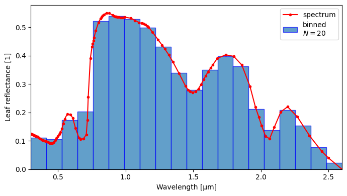
Leaf/soil optical properties
ds0_l = crt.data.load_ideal_leaf().dropna(dim="wl")
ds0_l
<xarray.Dataset> Size: 3kB
Dimensions:  (wl: 108)
Coordinates:
  * wl       (wl) float64 864B 0.3 0.305 0.31 0.315 0.32 ... 2.36 2.45 2.5 2.6
Data variables:
    rl       (wl) float64 864B 0.1253 0.1241 0.1229 ... 0.06321 0.03968 1e-10
tl (wl) float64 864B 0.08399 0.08376 0.08352 ... 0.0699 0.03549 1e-10bins2 = np.linspace(0.3, 2.6, 21)
ds1_l = crt.spectra.smear(ds0_l, bins2)
crt.spectra.plot_binned_ds(ds0_l, ds1_l, yname="rl")
Function crt1d.spectra.smear() can be applied to array-like, xarray.DataArray, or xarray.Dataset.
# `x` array must be provided if passing array
crt.spectra.smear(ds1_l.rl.values, bins2, x=ds1_l.wl)
array([0.05487465, 0.11476666, 0.16763666, 0.23817439, 0.48307759,
       0.53507554, 0.52547132, 0.49396821, 0.42819319, 0.34355597,
       0.29599888, 0.34741731, 0.38775264, 0.34816994, 0.22202369,
       0.15598805, 0.19195755, 0.15037308, 0.08022294, 0.01829059])
# `x` assumed to be the variable with `name` `'wl'`
crt.spectra.smear(ds1_l.rl, bins2)
<xarray.Dataset> Size: 488B
Dimensions:  (wl: 20, wle: 21)
Coordinates:
  * wl       (wl) float64 160B 0.3575 0.4725 0.5875 0.7025 ... 2.312 2.428 2.543
  * wle      (wle) float64 168B 0.3 0.415 0.53 0.645 ... 2.255 2.37 2.485 2.6
Data variables:
rl (wl) float64 160B 0.05487 0.1148 0.1676 ... 0.1504 0.08022 0.01829crt.spectra.smear(ds1_l, bins2)
<xarray.Dataset> Size: 648B
Dimensions:  (wl: 20, wle: 21)
Coordinates:
  * wl       (wl) float64 160B 0.3575 0.4725 0.5875 0.7025 ... 2.312 2.428 2.543
  * wle      (wle) float64 168B 0.3 0.415 0.53 0.645 ... 2.255 2.37 2.485 2.6
Data variables:
    rl       (wl) float64 160B 0.05487 0.1148 0.1676 ... 0.1504 0.08022 0.01829
tl (wl) float64 160B 0.04105 0.09165 0.1316 ... 0.1682 0.09196 0.01898Warning
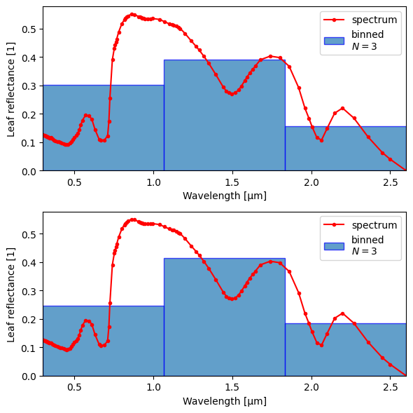
Smearing leaf/soil optical properties directly causes issues as well, though more subtle than for irradiance.
Reflectance/transmittance are like albedo in that they depend on the incoming light as well. We can account for this by weighting with a light spectrum when averaging the optical property spectra.
The influence of accounting for the incoming light spectrum is most apparent when the bins are large and few.
bins3 = np.linspace(0.3, 2.6, 4)

fig, axs = plt.subplots(2, 1, figsize=(6, 6))

for method, ax in zip(["tuv", "avg_optical_prop"], axs.flat):
    crt.spectra.plot_binned_ds(ds0_l, crt.spectra.smear(ds0_l, bins3, method=method), yname="rl", ax=ax)
Average optical properties
Below, we can see that when we compute the average reflectance, over certain regions the above doesn’t matter much (PAR/visible). In the NIR, however, there is a strong preference for smaller wavelengths, which overall weights leaf reflectance towards higher values.
In the below, 'uniform' corresponds to standard smearing, with no solar weighting.
First, we calculate average values using the original spectrum, loaded above.
# On the original leaf reflectance spectrum
boundss = [(0.4, 0.7), (0.7, 1.0), (1.0, 2.5), (0.3, 2.5)]
lights = ["planck", "uniform"]

for bounds in boundss:
    print(bounds)
    for light in lights:
        ybar = crt.spectra.avg_optical_prop(
            ds0_l.rl, bounds, x=ds0_l.wl, light=light
        )
        print(f" {light}: {ybar:.4g}")
(0.4, 0.7)
 planck: 0.1316
 uniform: 0.1317
(0.7, 1.0)
 planck: 0.4641
 uniform: 0.4812
(1.0, 2.5)
 planck: 0.3956
 uniform: 0.3017
(0.3, 2.5)
 planck: 0.2744
 uniform: 0.2944
Now, we use the spectrum smeared above.
# On a smeared/binned leaf reflectance spectrum
ds2 = crt.spectra.smear(ds0, bins2)
data = (
    ds2.sel(wl=ds1_l.wl.values, method="nearest").I_dr +
    ds2.sel(wl=ds1_l.wl.values, method="nearest").I_df
)
lights = ["planck", "uniform", data]

for bounds in boundss:
    print(bounds)
    for light in lights:
        ybar = crt.spectra.avg_optical_prop(
            ds1_l.rl, bounds, xe=ds1_l.wle, light=light
        )
        if isinstance(light, str):
            print(f" {light}: {ybar:.4g}")
        else:
            print(f" data: {ybar:.4g}")
(0.4, 0.7)
 planck: 0.1463
 uniform: 0.1492
 data: 0.1581
(0.7, 1.0)
 planck: 0.4401
 uniform: 0.4641
 data: 0.4382
(1.0, 2.5)
 planck: 0.3953
 uniform: 0.3016
 data: 0.3849
(0.3, 2.5)
 planck: 0.2754
 uniform: 0.2943
 data: 0.3197
👆 Notice that the values for 'uniform' and 'planck' are similar (though not identical) to the calculations on the pre-smeared spectrum.
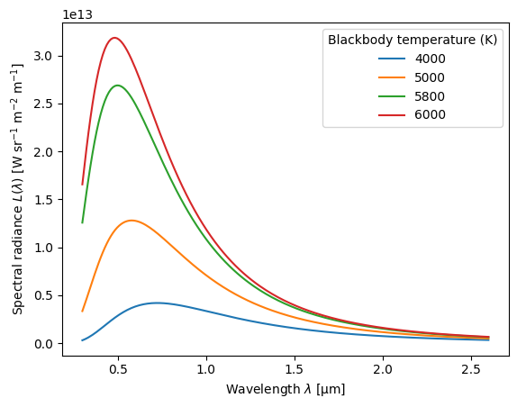
Planck function
Planck radiance is one of the light options can be used to weight values
when smearing the spectra with the method='avg_optical_prop' option. This is important for albedo, for example, because albedo in some waveband (such as visible or shortwave) depends on both the albedo spectrum and the spectrum of the illuminating light.
wl_um = np.linspace(0.3, 2.6, 200)
fig, ax = plt.subplots()
for T_K in [4000, 5000, 5800, 6000]:
    ax.plot(wl_um, crt.spectra.l_wl_planck(T_K, wl_um), label=T_K)
ax.set(
    xlabel=r"Wavelength $\lambda$ [μm]",
    ylabel=r"Spectral radiance $L(\lambda)$ [W sr$^{-1}$ m$^{-2}$ m$^{-1}$]",
)
ax.legend(title="Blackbody temperature (K)");