Leaf angles
from functools import partial

import matplotlib.pyplot as plt
import numpy as np
import pandas as pd
from scipy import optimize

import crt1d as crt
Leaf inclination angle distributions \(g(\theta_l)\)
named = {
    "spherical": crt.leaf_angle.g_spherical,
    "uniform": crt.leaf_angle.g_uniform,
    "planophile": crt.leaf_angle.g_planophile,
    "erectrophile": crt.leaf_angle.g_erectophile,
    "plagiophile": crt.leaf_angle.g_plagiophile,
}

theta_l = np.linspace(0, np.pi/2, 200)

fig, ax = plt.subplots()

for name, g_fn in named.items():
    ax.plot(np.rad2deg(theta_l), g_fn(theta_l), label=name)

ax.autoscale(True, "x", tight=True)
ax.set(
    xlabel=r"Leaf inclination angle $\theta_l$ [deg.]",
    ylabel="Probability density",
    title=r"$g(\theta_l)$ for various distributions",
)
ax.legend()
fig.tight_layout();
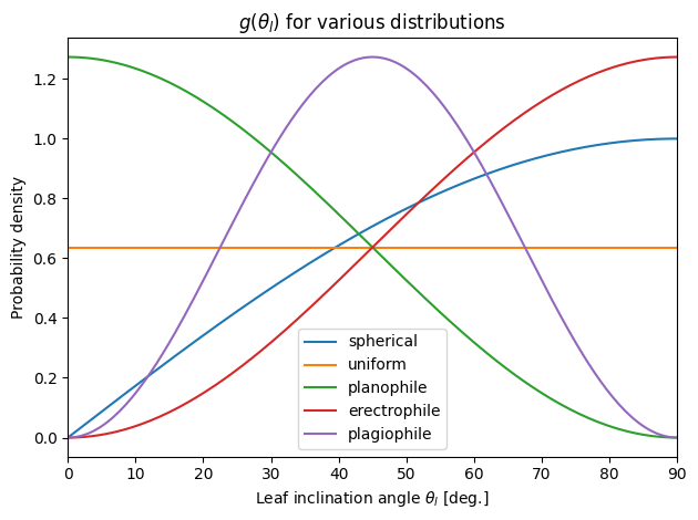
👆 Compare to Bonan (2019) Fig. 2.6.
Ellipsoidal
fig, ax = plt.subplots()

ellipsoidal_xs = [0.5, 1, 2, 4]

for x in ellipsoidal_xs:
    ax.plot(np.rad2deg(theta_l), crt.leaf_angle.g_ellipsoidal(theta_l, x), label=f"$x = {x}$")

ax.autoscale(True, "x", tight=True)
ax.set(
    xlabel=r"Leaf inclination angle $\theta_l$ [deg.]",
    ylabel="Probability density",
    title=r"$g(\theta_l)$ for different ellipsoidal distributions",
)
ax.legend()
fig.tight_layout();
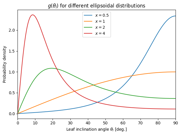
👆 Compare to Bonan (2019) Fig. 2.7. We can see that \(x = 1\) is the same as spherical in the previous figure. This makes sense since \(x\) is the ratio of the ellipsoid axes, \(b/a\). As \(x > 1\), the preference is for leaves that are only slightly inclined above the horizontal (oblate spheroid; left below). For \(x < 1\), we have a prolate spheroid and a preference for greater inclination angles.

Mean leaf angle from \(g(\theta_l)\)
df = pd.DataFrame(index=named.keys(), data={
    "mla_deg": [crt.leaf_angle.mla_from_g(g_fn) for g_fn in named.values()]
})

for x in ellipsoidal_xs:
    df.loc[f"ellipsoidal_x={x}", "mla_deg"] = crt.leaf_angle.mla_from_g(
        lambda theta_l: crt.leaf_angle.g_ellipsoidal(theta_l, x)
    )

df.round(3)
| mla_deg | |
|---|---|
| spherical | 57.296 |
| uniform | 45.000 |
| planophile | 26.762 |
| erectrophile | 63.238 |
| plagiophile | 45.000 |
| ellipsoidal_x=0.5 | 72.081 |
| ellipsoidal_x=1 | 57.296 |
| ellipsoidal_x=2 | 38.477 |
| ellipsoidal_x=4 | 21.983 |
👆 Note that the spherical leaf angle distribution’s mean leaf angle of \(\approx 57.3^\circ\) is properly recovered when \(x=1\) is used with the ellipsoidal \(g\).
There is a formula (Campbell 1990, eq. 16) that can be used to approximate the mean leaf angle for the ellipsoidal distribution without needing to numerically integrate \(g(\theta_l)\). Below we test it out.
fig, [ax1, ax2] = plt.subplots(2, 1, sharex=True, figsize=(6, 6))

x = np.linspace(0.01, 10, 200)

yhat = crt.leaf_angle.x_to_mla_approx(x)
y = np.array([crt.leaf_angle.x_to_mla_integ(xi) for xi in x])

ax1.plot(x, y, label="numerical integration of exact PDF")
ax1.plot(x, yhat, label="approximation formula")

ax2.plot(x, yhat - y, c="0.2", label="approx. minus integ.")
ax2.axhline(0, c="0.7", lw=1)

ax1.set(ylabel="Mean leaf angle [deg.]", title="Ellipsoidal mean leaf angle from $x$")
ax2.set(xlabel="$x$ (spheroid axis ratio)", ylabel="Mean leaf angle [deg.]")
ax1.legend()
ax2.legend()
fig.tight_layout();
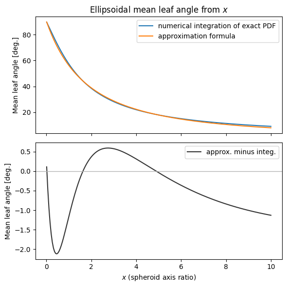
The nice thing about the approximate formula is that we can invert it and obtain \(x\) from mean leaf angle. Of course, we can also do this numerically.
mlas = [10, 20, 50, 57.296, 60, 80]

df = pd.DataFrame({
    "mla_deg": mlas,
    "x_approx": [crt.leaf_angle.mla_to_x_approx(mla) for mla in mlas],
    "x_integ": [crt.leaf_angle.mla_to_x_integ(mla) for mla in mlas],
})

df.round(3)
| mla_deg | x_approx | x_integ | |
|---|---|---|---|
| 0 | 10.000 | 8.380 | 9.153 |
| 1 | 20.000 | 4.477 | 4.441 |
| 2 | 50.000 | 1.291 | 1.316 |
| 3 | 57.296 | 0.951 | 1.000 |
| 4 | 60.000 | 0.842 | 0.897 |
| 5 | 80.000 | 0.227 | 0.274 |
\(\chi_l\)
This index characterizes the departure of the leaf angle distribution from spherical. Vertical leaves have \(\chi_l = -1\) and horizontal leaves \(\chi_l = +1\).
df = pd.DataFrame(index=named.keys(), data={
    "xl": [crt.leaf_angle.xl_from_g(g_fn) for g_fn in named.values()]
})

for x in ellipsoidal_xs:
    df.loc[f"ellipsoidal_x={x}", "xl"] = crt.leaf_angle.xl_from_g(
        lambda theta_l: crt.leaf_angle.g_ellipsoidal(theta_l, x)
    )

df.round(3)
| xl | |
|---|---|
| spherical | 0.000 |
| uniform | 0.211 |
| planophile | 0.527 |
| erectrophile | -0.115 |
| plagiophile | 0.313 |
| ellipsoidal_x=0.5 | -0.326 |
| ellipsoidal_x=1 | -0.000 |
| ellipsoidal_x=2 | 0.354 |
| ellipsoidal_x=4 | 0.638 |
\(G(\psi)\)
Most of the time we use the ellipsoidal \(G(\psi)\). In the canopy RT schemes, this is used for constructing \(K_b(\psi)\) and also used directly by some schemes.
fig, [[ax1, ax2], [ax3, ax4]] = plt.subplots(2, 2, figsize=(10, 7))

ax1.sharey(ax2)

sza = np.linspace(0, 89, 200)
psi = np.deg2rad(sza)
mu = np.cos(psi)

for x in ellipsoidal_xs:
    approx = crt.leaf_angle.G_ellipsoidal_approx(psi, x)
    exact = crt.leaf_angle.G_ellipsoidal(psi, x)

    l, = ax1.plot(sza, approx, ":", lw=3, label=f"approx., $x={x}$")
    c = c=l.get_color()
    ax1.plot(sza, exact, label=f"analytical, $x={x}$", c=c)
    ax2.plot(mu, exact, c=c)
    ax3.plot(sza, approx - exact, c=c)
    ax4.plot(mu, exact/mu, c=c)

# Horizontal/vertical limits for reference
for name, G_fn, color, lw in [
    ("horizontal", crt.leaf_angle.G_horizontal, "0.25", 0.8),
    ("vertical", crt.leaf_angle.G_vertical, "0.75", 1),
]:
    G = G_fn(psi)
    ax1.plot(sza, G, c=color, lw=lw, zorder=0, label=name)
    ax2.plot(mu, G, c=color, lw=lw, zorder=0)
    ax4.plot(mu, G/mu, c=color, lw=lw, zorder=0)

ax1.set(xlabel=r"Solar zenith angle $\psi$ [deg.]", ylabel="$G$", title="Ellipsoidal $G$ vs SZA")

ax2.set(xlabel=r"$\mu = \cos \psi$", ylabel="$G$", title=r"Ellipsoidal $G$ vs $\mu$")

ax3.set(xlabel=r"Solar zenith angle $\psi$ [deg.]", ylabel=r"$\delta G$", title="Approx. minus analytical")
ax3.axhline(0, ls=":", c="0.7", lw=1)

ax4.set(xlabel=r"$\mu = \cos \psi$", ylabel="$K_b$", title=r"$K_b = G/\mu$ vs $\mu$", ylim=(None, 5))

for ax in [ax1, ax2, ax4]:
    ax.set_ylim(ymin=0)

for ax in fig.get_axes():
    ax.autoscale(True, "x", tight=True)

fig.legend(bbox_to_anchor=(0.98, 0.5), loc="center left")
fig.tight_layout();
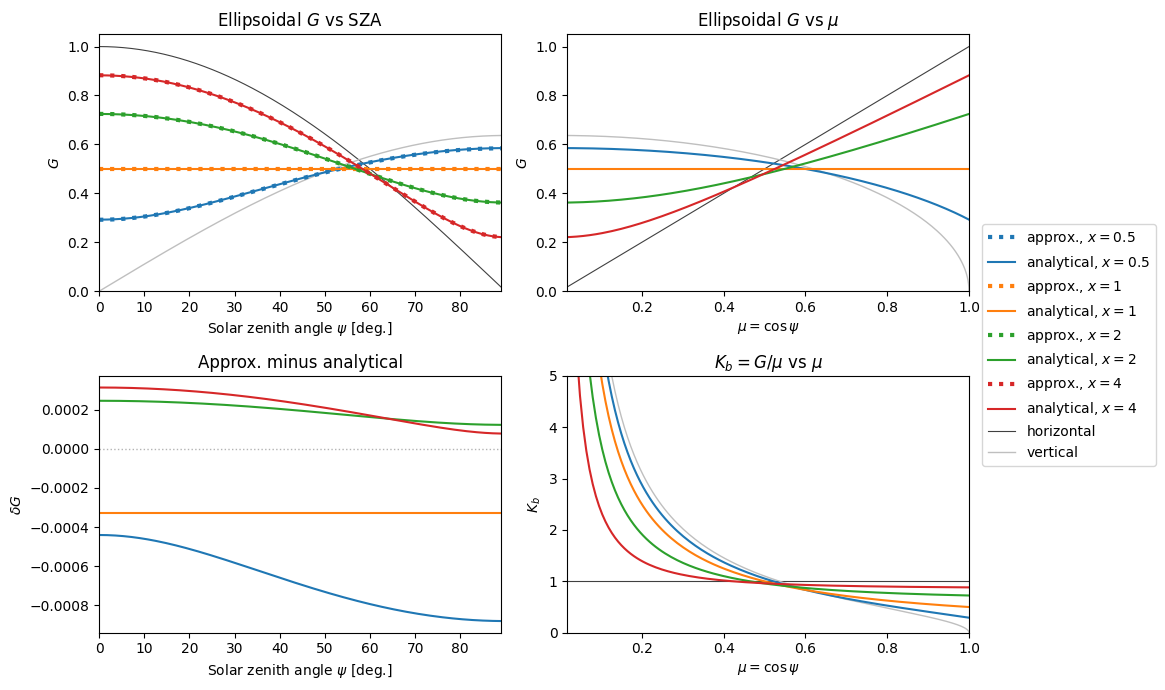
👆 The bottom right panel can be compared to Bonan (2019) Fig. 14.9, although that figure’s \(x\) coordinate is SZA (degrees) instead of \(\mu\).
In the top left panel, note that although each curve (aside from \(x = 1\)) does cross \(G = 0.5\), they do this at different values of SZA.
Where does \(G = 0.5\)?
For spherical, \(G = 0.5\) for all SZA. But for the others, it varies.
data = []
for x in ellipsoidal_xs + [0.1, 3, 10]:
    if x == 1:
        continue

    G_fn = partial(crt.leaf_angle.G_ellipsoidal, x=x)

    def f(sza):
        psi = np.deg2rad(sza)
        G = G_fn(psi)
        return G - 0.5

    sol = optimize.root_scalar(f, x0=60, bracket=(45, 75), method="bisect", xtol=1e-5)

    data.append((f"ellipsoidal x={x}", sol.root))

data.append(("vertical (analytical)", np.rad2deg(np.arcsin(np.pi/4))))
data.append(("horizontal (analytical)", np.rad2deg(np.arccos(0.5))))

df = pd.DataFrame(data, columns=["G fn", "SZA"])
df["psi"] = np.deg2rad(df["SZA"])
df["mu"] = np.cos(df["psi"])
(
    df
    .set_index("G fn")
    .sort_values("SZA")
)
| SZA | psi | mu | |
|---|---|---|---|
| G fn | |||
| vertical (analytical) | 51.757519 | 0.903339 | 0.618991 |
| ellipsoidal x=0.1 | 51.868823 | 0.905282 | 0.617464 |
| ellipsoidal x=0.5 | 53.157227 | 0.927769 | 0.599621 |
| ellipsoidal x=2 | 56.687529 | 0.989384 | 0.549205 |
| ellipsoidal x=3 | 57.718384 | 1.007376 | 0.534081 |
| ellipsoidal x=4 | 58.322604 | 1.017921 | 0.525136 |
| ellipsoidal x=10 | 59.483564 | 1.038184 | 0.507786 |
| horizontal (analytical) | 60.000000 | 1.047198 | 0.500000 |
👆 “SZA” and “psi” (\(\psi\)) above are both the solar zenith angle, but the former is in degrees while the latter is in radians. “mu”: \(\mu = \cos{\psi}\).
Where does \(K_b = 1\)?
For horizontal (\(G(\psi) = \cos{\psi}\)), \(K_b = 1\) for all SZA. But for the others, it varies.
data = []
for x in ellipsoidal_xs + [0.1, 3, 10]:

    G_fn = partial(crt.leaf_angle.G_ellipsoidal, x=x)

    def f(sza):
        psi = np.deg2rad(sza)
        G = G_fn(psi)
        return G / np.cos(psi) - 1

    sol = optimize.root_scalar(f, x0=60, bracket=(45, 75), method="bisect", xtol=1e-5)

    data.append((f"ellipsoidal x={x}", sol.root))

data.append(("vertical (analytical)", np.rad2deg(np.arctan(np.pi/2))))
data.append(("spherical (analytical)", np.rad2deg(np.arccos(0.5))))

df = pd.DataFrame(data, columns=["G fn", "SZA"])
df["psi"] = np.deg2rad(df["SZA"])
df["mu"] = np.cos(df["psi"])
(
    df
    .set_index("G fn")
    .sort_values("SZA")
)
| SZA | psi | mu | |
|---|---|---|---|
| G fn | |||
| vertical (analytical) | 57.518363 | 1.003885 | 0.537029 |
| ellipsoidal x=0.1 | 57.585490 | 1.005056 | 0.536041 |
| ellipsoidal x=0.5 | 58.540299 | 1.021721 | 0.521899 |
| spherical (analytical) | 60.000000 | 1.047198 | 0.500000 |
| ellipsoidal x=1 | 60.000007 | 1.047198 | 0.500000 |
| ellipsoidal x=2 | 62.272518 | 1.086860 | 0.465267 |
| ellipsoidal x=3 | 63.793538 | 1.113407 | 0.441607 |
| ellipsoidal x=4 | 64.872959 | 1.132247 | 0.424627 |
| ellipsoidal x=10 | 67.969158 | 1.186286 | 0.375106 |